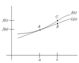
One of the important applications
of the derivative at a point is to use it to approximate the value of a
function at nearby points. This works because within a sufficiently
small interval around the point, the function can be approximated by a
tangent line through the point.

Point A has coordinates (a,
f(a))
and is on the curve y = f(x). A tangent line,
L(x)
passes through point A. The slope of this tangent line is the derivative
of f(x) at x = a, or
f (a).
Then we can show, using the point-slope form of a line that
If a value of x is sufficiently
close to a, then the value of y on the line L(x)
will be very close to the value of y on the graph of f(x).
That is, points B and C have almost the same value of y
if they have the same value of x. Therefore, we say that the
tangent line L(x) is a linear approximation to the function
f(x)
for values of x sufficiently close to a.
The error, that is f(x)
L(x) depends on x, hence it too is a function of
x.
This error function can be written as
The percentage error is

Example 1: Use a linear
approximation near x = 3 to estimate the value of f(3.1)
if f(x) = x2.
Solution: Here,
a
= 3, f(3) = 9, and x = 3.1. Also, for our function, f(x)
= 2x
which means that f '(a)
= f '(3) = 6. Therefore, the equation of the tangent line is

Thus we are saying that f(3.1) »
9.6. How good is this? Well, substituting into the real function
gives f (3.1) = 3.1 2 = 9.61. The error function
is f(x) L(x) = 0.01

The percent error is

which is pretty good!
First, we will define the following function:
